Numerical accuracy: time stepping

GRLP integrates the sediment-conservation equation with a semi-implicit scheme. By default it is second-order in time (BDF2) and second-order in space, and runs the semi-implicit iteration to convergence each step. The first-order backward-Euler scheme is available with set_time_integration(1). This page shows what the time-stepping error looks like for each, why second order is the default, and how to choose a step.

How the accuracy is measured

By self-convergence. We run the same scenario — a river adjusting to a step increase in uplift — first with a very short time step, which we treat as “the truth,” then again with a series of progressively longer steps, and measure how far each longer-step run lands from the truth. The scenario is run only part way to its new steady state (one equilibration time, after Paola et al., 1992), because at steady state the answer no longer depends on the time step and the comparison would be empty. The same setup is checked automatically by tests/test_time_accuracy.py, and the figure below is regenerated by docs/accuracy_figure.py.

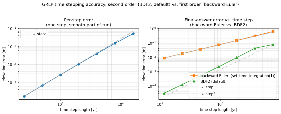
Elevation error as the time step lengthens, on log–log axes. Left: the error from a single step, measured in a smoothly-evolving part of the run. Right: the error in the final profile after a whole run to a fixed end time, for the default BDF2 scheme (∝ step²) and the first-order backward-Euler option (∝ step).

What the figure says

Per step (left). A single step of length Δt lands off the truth by an amount that grows like Δt²:

one step of…	is off by…
1,000 yr	0.26 mm
4,000 yr	3.9 mm
16,000 yr	51 mm

Double the step → roughly quadruple the error in that step.

Final answer (right). Over a whole run to a fixed end time, the first-order backward-Euler option’s error in the final profile grows like Δt:

step length	error in final profile (backward Euler)
~1,200 yr	~0.008 m
~9,400 yr	~0.07 m
~75,000 yr	~0.6 m

Double the step → roughly double the final error. The default BDF2 scheme (green curve) instead grows like Δt² — far smaller, especially at large steps (see below).

Why the two differ by one power. A single step’s error is quadratic, but a smaller step means proportionally more steps, so the little per-step errors accumulate over more of them: (T / Δt) steps × Δt² each = T · Δt, i.e. linear. So per step the accuracy degrades quadratically, while the accuracy of the final answer — the thing a modeller cares about — degrades linearly with step length for backward Euler. That linear-in-Δt behaviour is what “first-order in time” means; BDF2 removes it, leaving the Δt² scaling below.

Choosing a time step

With the default BDF2 the final error is proportional to Δt², so halving the step quarters the error — you reach a target accuracy at a much larger step than backward Euler would need. Pick Δt from the accuracy you need relative to the elevation changes you are resolving; for the transient above, BDF2 holds the final error at the centimetre level with steps of tens of thousands of years. With the backward-Euler option the error is proportional to Δt instead, so it needs proportionally smaller steps for the same accuracy.

Second order in time: BDF2 (the default)

First order ties accuracy to cost tightly: to cut the final error by 10×, you must cut Δt by 10× — ten times as many steps. GRLP therefore integrates in time with BDF2 by default, which makes the final error scale like Δt² instead of Δt — the green curve in the figure above. So for a target accuracy you can take a substantially larger step (roughly an order of magnitude) and run transients much more cheaply with no loss of fidelity; equivalently, at the same step BDF2 is far more accurate (about 7× smaller final error at a 75,000-yr step in the figure, and the gap widens as steps grow).

BDF2 is L-stable — it damps sharp transients rather than ringing — bootstraps its first step with backward Euler, and reaches its second-order rate once the semi-implicit iteration is converged (the default, below). Steady states are independent of the time step, so the scheme only affects the path through time. The two schemes also agree as Δt → 0: they differ only by their finite-step truncation error, so on a well-resolved run the choice barely matters — BDF2 simply reaches that well-resolved answer at a much larger step. To fall back to first-order backward Euler:

lp.set_time_integration(1)      # 2 = BDF2 (default), 1 = backward Euler

(also available on Network). See MNiMORPH/GRLP#16.

Iterating the solve to convergence (the default)

Each step is semi-implicit: GRLP relinearizes and re-solves a few times (Picard iteration). By default it iterates to convergence — until the inter-iteration elevation change max|z_k − z_{k-1}| falls below a tolerance (default 0.1 mm) — so a step is as converged as its second-order accuracy needs, without your having to guess an iteration count:

lp.set_iteration_tolerance(1e-4)   # the default: iterate until change < 0.1 mm

The iteration is capped at max_iter, and warns if it reaches the cap without converging. That happens for a very large step: the fixed-point (Picard) iteration is only a contraction when the step is small enough, so past that it plateaus rather than converging. The warning is the signal to take a smaller step (or accept the reported residual); the run itself still relaxes to the correct steady state.

If you know how many iterations a step needs, fixing the count is a little faster:

lp.set_niter(3)                    # fixed 3 iterations per step (expert option)

Setting a tolerance and setting niter are mutually exclusive — the most recent call wins. See MNiMORPH/GRLP#17.

Adaptive time stepping (opt-in)

Everything above uses a fixed step you choose. But a transient is rarely uniform in time: it changes fast just after a perturbation and slowly as it settles, so a single step is either too small late or too large early. Adaptive stepping picks the step size for you — small where the profile moves fast, large where it is smooth — to hold a target accuracy:

lp.set_time_integration(2)          # adaptive stepping uses BDF2
lp.set_adaptive_timestep(1e-3)      # per-step error tolerance, in metres
lp.evolve_threshold_width_river_adaptive(T)   # advance a total time T

Instead of a step count and a step length, you give a total time T and a tolerance tol. Each candidate step is checked by step doubling — the step is taken once at Δt and again as two steps of Δt/2, and the difference between the two estimates the error. If it exceeds tol the step is rejected and retried smaller; otherwise it is accepted (advancing with the more accurate half-step solution) and the next step grows toward the largest size that still meets tol. The first step is bootstrapped with an error-controlled backward-Euler step, so the result does not depend on any initial-step guess.

As with an ODE solver’s tolerance, tol bounds the per-step error; the total path error is of comparable magnitude, and tightening tol reduces it monotonically (at the cost of more, smaller steps). Pair with set_iteration_tolerance so the nonlinear solve the estimate relies on is itself converged. See MNiMORPH/GRLP#16.

Adaptive stepping is a convenience, not a speed-up. For GRLP it is slower than a well-chosen fixed BDF2 step, not faster: benchmarking (benchmarks/adaptive_timestep_benchmark.py) shows it costs several times more linear solves at matched accuracy — roughly 4× for a smooth uplift-step transient and over 10× for a sharper base-level drop. The reason is that GRLP’s governing equation is diffusive, so its transients are smooth in time: uniform steps are already close to the optimal placement, and the extra solves that step doubling spends to estimate the error each step are never repaid by better placement. Reach for adaptive stepping when you want to set an accuracy and let the solver find the step — not to run faster. When speed matters, use a fixed BDF2 step (the second-order option above buys far more than adaptivity does).