GRLP river networks: a 5-segment example

The single-profile tutorial (example_1d) evolved one river long profile. GRLP also solves whole river networks — in fact every GRLP solution is a network solution, and a single profile is just the trivial one-edge case.

In a network, segments (reaches) meet at confluences, where two rules hold:

1. Sediment and water sum: a segment’s supply is the sum of its upstream tributaries’.

2. Elevation is continuous across the junction.

The solver assembles one global system over the whole network by walking the topology, then solves it just as for a single segment. Here we build a small 5-segment network — two confluences — by hand, evolve it to steady state, and plot it. Compare each step with the single-profile tutorial.

Reference: McNab et al. (2025, ESurf) develop and apply the network-scale theory.

import numpy as np
from matplotlib import pyplot as plt

import grlp

1. Wire up the topology

A network is defined by how its segments connect. Each segment lists its upstream and downstream neighbours by ID. Channel heads have no upstream segments; the outlet has no downstream segment.

Our little network (heads 0, 1, 3):

head 0 ─┐
        ├─ segment 2 ─┐
head 1 ─┘             ├─ segment 4 ──▶ outlet (base level)
head 3 ──────────────┘

# Each segment's upstream / downstream neighbours, by ID.
# heads 0, 1 join at 2;  segment 2 and head 3 join at 4;  4 is the outlet.
upstream_segment_IDs   = [[], [], [0, 1], [], [2, 3]]
downstream_segment_IDs = [[2], [2], [4], [4], []]

2. Give each segment geometry and discharge

Every segment carries its own arrays: node positions x (downstream distance), initial bed z, discharge Q, and valley width B. Discharge grows downstream as tributaries join — here the two headwater segments each carry 5 m³/s, so their trunk (segment 2) carries 10, and adding head 3 (10 m³/s) makes the outlet trunk (segment 4) carry 20.

One rule to remember: a confluence segment needs at least 3 nodes (the conservative junction cell reaches two nodes in from the boundary). Valley width is uniform here to keep the example simple.

numel = [5, 7, 4, 8, 6]        # nodes per segment; confluence segments need >= 3

# Downstream distance [m] of each node, per segment (a small dendritic layout)
x = [ 1000. * np.array([2, 4, 6.5, 9, 10]),
      1000. * np.array([0, 1, 2, 3, 6, 8, 10.5]),
      1000. * np.array([12, 15, 18, 20]),
      1000. * np.array([2, 6, 8, 12, 14, 16, 18, 20]),
      1000. * np.array([23, 24, 27, 29, 29.5, 30]) ]

# Discharge [m3/s], constant within each segment and summing at confluences:
#   heads 0,1 (5 + 5) -> trunk 2 (10);  trunk 2 + head 3 (10 + 10) -> outlet 4 (20)
Q_in = [5., 5., 10., 10., 20.]

z = [np.zeros(n) for n in numel]                  # start flat
Q = [q * np.ones(n) for q, n in zip(Q_in, numel)]
B = [100. * np.ones(n) for n in numel]            # uniform valley width [m]

3. Boundary conditions

Same idea as the single profile, applied at the network’s edges:

• Upstream — each channel head gets an equilibrium slope S0 (here 1.5%), which sets that head’s sediment supply (exactly as set_S0 does for one profile).

• Downstream — the outlet has a base level, the point (x_bl, z_bl) (recall set_bl from the 1-D tutorial). The network places it on its single river mouth.

S0 = [0.015, 0.015, 0.015]   # equilibrium slope at each channel head (0, 1, 3)
x_bl = 1000. * 32            # base-level position [m]
z_bl = 0.                    # base-level elevation [m]

4. Build and evolve

Instantiate a Network, pass everything through initialize(), then evolve to steady state — the same kind of evolve_* call as a single profile, now over the whole graph. (get_z_lengths() tells the solver how many nodes each segment has before the first solve.)

net = grlp.Network()
net.initialize(
    config_file=None,
    x_bl=x_bl, z_bl=z_bl,
    S0=S0, Q_s_0=None,
    upstream_segment_IDs=upstream_segment_IDs,
    downstream_segment_IDs=downstream_segment_IDs,
    x=x, z=z, Q=Q, B=B,
    overwrite=False,
)
net.set_niter(3)
net.get_z_lengths()
net.evolve_threshold_width_river_network(nt=100, dt=1e11)

5. Plot the network

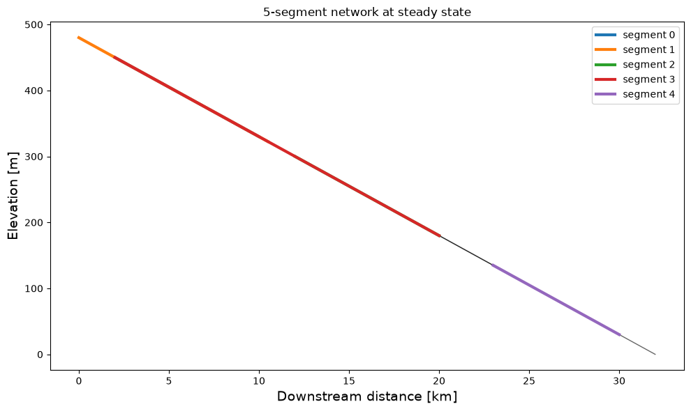
Each segment is drawn in its own colour; the thin black lines are the connectors — a segment’s downstream end joining its neighbour across each confluence, and the outlet joining base level. The profiles are concave-up, descend to base level, and steepen in the smaller-discharge headwaters.

plt.figure(figsize=(10, 6))
for lp in net.segments:
    # connector: downstream end -> neighbour across the junction
    # (or, at the outlet, down to base level)
    if len(lp.downstream_segment_IDs) > 0:
        ds = net.segments[lp.downstream_segment_IDs[0]]
        plt.plot([lp.x[-1] / 1000., ds.x[0] / 1000.],
                 [lp.z[-1], ds.z[0]], 'k-', lw=1, alpha=0.6)
    else:
        plt.plot([lp.x[-1] / 1000., lp.x_ghost_downstream / 1000.],
                 [lp.z[-1], lp.z_bl], 'k-', lw=1, alpha=0.6)
    plt.plot(lp.x / 1000., lp.z, '-', lw=3, label='segment %d' % lp.ID)
plt.xlabel('Downstream distance [km]', fontsize=14)
plt.ylabel('Elevation [m]', fontsize=14)
plt.title('5-segment network at steady state')
plt.legend()
plt.tight_layout()
plt.show()

Next steps

You built a network by hand. To generate networks at scale — random topologies with no DEM required, plus network-structure analysis (Hack’s law, Strahler orders, Horton ratios) — see the random-network tutorial (example_random_network).

Full documentation and API reference: grlp.readthedocs.io.