GRLP random networks: generate and analyze at scale
The hand-built 5-segment network showed the mechanics of confluences. This capstone does two things that only make sense at scale:
Generate a whole river network with no DEM required — a random Shreve (1966, 1974) binary tree, wired up with discharges and widths automatically.
Analyze its structure — Strahler stream orders, Horton ratios, and Hack-type scaling — the descriptors that characterize real drainage networks.
This is the quickest way to get a runnable GRLP network for experiments. Reference: McNab et al. (2025, ESurf).
import random

import numpy as np
from matplotlib import pyplot as plt

import grlp

# Seed both RNGs for a reproducible network; drop these to draw a new one.
random.seed(7)
np.random.seed(7)
1. Generate a Shreve random network
generate_random_network builds the topology and populates it with node spacing, discharges (accumulating downstream), and valley widths. The main knobs:
magnitude— the number of channel heads (the network’s “size”).max_length— the length of the longest source-to-outlet path [m].mean_discharge— sets segment discharges from drainage area.
It returns the Network and its topology object.
net, topo = grlp.generate_random_network(
    magnitude=8,
    max_length=2.0e4,
    mean_discharge=10.,
)
net.set_niter(3)
net.get_z_lengths()
print('%d segments, %d channel heads'
      % (len(net.segments),
         len(net.list_of_channel_head_segment_IDs)))
15 segments, 8 channel heads
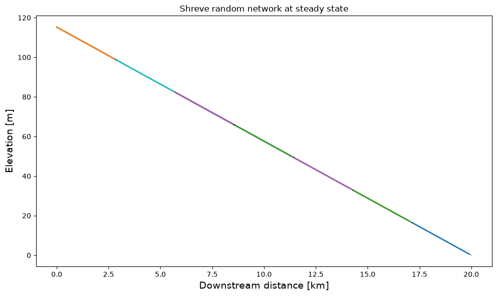
2. Evolve to steady state and plot the long profiles
Exactly as for the hand-built network — one call evolves the whole graph.
net.evolve_threshold_width_river_network(nt=200, dt=3.15e11)

plt.figure(figsize=(10, 6))
for lp in net.segments:
    if lp.downstream_segment_IDs:
        ds = net.segments[lp.downstream_segment_IDs[0]]
        plt.plot([lp.x[-1] / 1000., ds.x[0] / 1000.],
                 [lp.z[-1], ds.z[0]], 'k-', lw=1, alpha=0.5)
    else:
        plt.plot([lp.x[-1] / 1000., lp.x_ghost_downstream / 1000.],
                 [lp.z[-1], lp.z_bl], 'k-', lw=1, alpha=0.5)
    plt.plot(lp.x / 1000., lp.z, '-', lw=2)
plt.xlabel('Downstream distance [km]', fontsize=14)
plt.ylabel('Elevation [m]', fontsize=14)
plt.title('Shreve random network at steady state')
plt.tight_layout()
plt.show()
3. The network planform
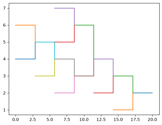
Network.plot() draws the branching map view — the dendritic pattern of the random tree.
net.plot()
{0: {'x': array([17.14285714, 17.24489796, 17.34693878, 17.44897959, 17.55102041,
         17.65306122, 17.75510204, 17.85714286, 17.95918367, 18.06122449,
         18.16326531, 18.26530612, 18.36734694, 18.46938776, 18.57142857,
         18.67346939, 18.7755102 , 18.87755102, 18.97959184, 19.08163265,
         19.18367347, 19.28571429, 19.3877551 , 19.48979592, 19.59183673,
         19.69387755, 19.79591837, 19.89795918, 20.        , 20.        ]),
  'y': array([2., 2., 2., 2., 2., 2., 2., 2., 2., 2., 2., 2., 2., 2., 2., 2., 2.,
         2., 2., 2., 2., 2., 2., 2., 2., 2., 2., 2., 2., 2.])},
 1: {'x': array([14.28571429, 14.3877551 , 14.48979592, 14.59183673, 14.69387755,
         14.79591837, 14.89795918, 15.        , 15.10204082, 15.20408163,
         15.30612245, 15.40816327, 15.51020408, 15.6122449 , 15.71428571,
         15.81632653, 15.91836735, 16.02040816, 16.12244898, 16.2244898 ,
         16.32653061, 16.42857143, 16.53061224, 16.63265306, 16.73469388,
         16.83673469, 16.93877551, 17.04081633, 17.14285714, 17.14285714]),
  'y': array([1., 1., 1., 1., 1., 1., 1., 1., 1., 1., 1., 1., 1., 1., 1., 1., 1.,
         1., 1., 1., 1., 1., 1., 1., 1., 1., 1., 1., 1., 2.])},
 2: {'x': array([14.28571429, 14.3877551 , 14.48979592, 14.59183673, 14.69387755,
         14.79591837, 14.89795918, 15.        , 15.10204082, 15.20408163,
         15.30612245, 15.40816327, 15.51020408, 15.6122449 , 15.71428571,
         15.81632653, 15.91836735, 16.02040816, 16.12244898, 16.2244898 ,
         16.32653061, 16.42857143, 16.53061224, 16.63265306, 16.73469388,
         16.83673469, 16.93877551, 17.04081633, 17.14285714, 17.14285714]),
  'y': array([3., 3., 3., 3., 3., 3., 3., 3., 3., 3., 3., 3., 3., 3., 3., 3., 3.,
         3., 3., 3., 3., 3., 3., 3., 3., 3., 3., 3., 3., 2.])},
 3: {'x': array([11.42857143, 11.53061224, 11.63265306, 11.73469388, 11.83673469,
         11.93877551, 12.04081633, 12.14285714, 12.24489796, 12.34693878,
         12.44897959, 12.55102041, 12.65306122, 12.75510204, 12.85714286,
         12.95918367, 13.06122449, 13.16326531, 13.26530612, 13.36734694,
         13.46938776, 13.57142857, 13.67346939, 13.7755102 , 13.87755102,
         13.97959184, 14.08163265, 14.18367347, 14.28571429, 14.28571429]),
  'y': array([2., 2., 2., 2., 2., 2., 2., 2., 2., 2., 2., 2., 2., 2., 2., 2., 2.,
         2., 2., 2., 2., 2., 2., 2., 2., 2., 2., 2., 2., 3.])},
 4: {'x': array([11.42857143, 11.53061224, 11.63265306, 11.73469388, 11.83673469,
         11.93877551, 12.04081633, 12.14285714, 12.24489796, 12.34693878,
         12.44897959, 12.55102041, 12.65306122, 12.75510204, 12.85714286,
         12.95918367, 13.06122449, 13.16326531, 13.26530612, 13.36734694,
         13.46938776, 13.57142857, 13.67346939, 13.7755102 , 13.87755102,
         13.97959184, 14.08163265, 14.18367347, 14.28571429, 14.28571429]),
  'y': array([4., 4., 4., 4., 4., 4., 4., 4., 4., 4., 4., 4., 4., 4., 4., 4., 4.,
         4., 4., 4., 4., 4., 4., 4., 4., 4., 4., 4., 4., 3.])},
 5: {'x': array([ 8.57142857,  8.67346939,  8.7755102 ,  8.87755102,  8.97959184,
          9.08163265,  9.18367347,  9.28571429,  9.3877551 ,  9.48979592,
          9.59183673,  9.69387755,  9.79591837,  9.89795918, 10.        ,
         10.10204082, 10.20408163, 10.30612245, 10.40816327, 10.51020408,
         10.6122449 , 10.71428571, 10.81632653, 10.91836735, 11.02040816,
         11.12244898, 11.2244898 , 11.32653061, 11.42857143, 11.42857143]),
  'y': array([3., 3., 3., 3., 3., 3., 3., 3., 3., 3., 3., 3., 3., 3., 3., 3., 3.,
         3., 3., 3., 3., 3., 3., 3., 3., 3., 3., 3., 3., 4.])},
 6: {'x': array([5.71428571, 5.81632653, 5.91836735, 6.02040816, 6.12244898,
         6.2244898 , 6.32653061, 6.42857143, 6.53061224, 6.63265306,
         6.73469388, 6.83673469, 6.93877551, 7.04081633, 7.14285714,
         7.24489796, 7.34693878, 7.44897959, 7.55102041, 7.65306122,
         7.75510204, 7.85714286, 7.95918367, 8.06122449, 8.16326531,
         8.26530612, 8.36734694, 8.46938776, 8.57142857, 8.57142857]),
  'y': array([2., 2., 2., 2., 2., 2., 2., 2., 2., 2., 2., 2., 2., 2., 2., 2., 2.,
         2., 2., 2., 2., 2., 2., 2., 2., 2., 2., 2., 2., 3.])},
 7: {'x': array([5.71428571, 5.81632653, 5.91836735, 6.02040816, 6.12244898,
         6.2244898 , 6.32653061, 6.42857143, 6.53061224, 6.63265306,
         6.73469388, 6.83673469, 6.93877551, 7.04081633, 7.14285714,
         7.24489796, 7.34693878, 7.44897959, 7.55102041, 7.65306122,
         7.75510204, 7.85714286, 7.95918367, 8.06122449, 8.16326531,
         8.26530612, 8.36734694, 8.46938776, 8.57142857, 8.57142857]),
  'y': array([4., 4., 4., 4., 4., 4., 4., 4., 4., 4., 4., 4., 4., 4., 4., 4., 4.,
         4., 4., 4., 4., 4., 4., 4., 4., 4., 4., 4., 4., 3.])},
 8: {'x': array([2.85714286, 2.95918367, 3.06122449, 3.16326531, 3.26530612,
         3.36734694, 3.46938776, 3.57142857, 3.67346939, 3.7755102 ,
         3.87755102, 3.97959184, 4.08163265, 4.18367347, 4.28571429,
         4.3877551 , 4.48979592, 4.59183673, 4.69387755, 4.79591837,
         4.89795918, 5.        , 5.10204082, 5.20408163, 5.30612245,
         5.40816327, 5.51020408, 5.6122449 , 5.71428571, 5.71428571]),
  'y': array([3., 3., 3., 3., 3., 3., 3., 3., 3., 3., 3., 3., 3., 3., 3., 3., 3.,
         3., 3., 3., 3., 3., 3., 3., 3., 3., 3., 3., 3., 4.])},
 9: {'x': array([2.85714286, 2.95918367, 3.06122449, 3.16326531, 3.26530612,
         3.36734694, 3.46938776, 3.57142857, 3.67346939, 3.7755102 ,
         3.87755102, 3.97959184, 4.08163265, 4.18367347, 4.28571429,
         4.3877551 , 4.48979592, 4.59183673, 4.69387755, 4.79591837,
         4.89795918, 5.        , 5.10204082, 5.20408163, 5.30612245,
         5.40816327, 5.51020408, 5.6122449 , 5.71428571, 5.71428571]),
  'y': array([5., 5., 5., 5., 5., 5., 5., 5., 5., 5., 5., 5., 5., 5., 5., 5., 5.,
         5., 5., 5., 5., 5., 5., 5., 5., 5., 5., 5., 5., 4.])},
 10: {'x': array([0.        , 0.10204082, 0.20408163, 0.30612245, 0.40816327,
         0.51020408, 0.6122449 , 0.71428571, 0.81632653, 0.91836735,
         1.02040816, 1.12244898, 1.2244898 , 1.32653061, 1.42857143,
         1.53061224, 1.63265306, 1.73469388, 1.83673469, 1.93877551,
         2.04081633, 2.14285714, 2.24489796, 2.34693878, 2.44897959,
         2.55102041, 2.65306122, 2.75510204, 2.85714286, 2.85714286]),
  'y': array([4., 4., 4., 4., 4., 4., 4., 4., 4., 4., 4., 4., 4., 4., 4., 4., 4.,
         4., 4., 4., 4., 4., 4., 4., 4., 4., 4., 4., 4., 5.])},
 11: {'x': array([0.        , 0.10204082, 0.20408163, 0.30612245, 0.40816327,
         0.51020408, 0.6122449 , 0.71428571, 0.81632653, 0.91836735,
         1.02040816, 1.12244898, 1.2244898 , 1.32653061, 1.42857143,
         1.53061224, 1.63265306, 1.73469388, 1.83673469, 1.93877551,
         2.04081633, 2.14285714, 2.24489796, 2.34693878, 2.44897959,
         2.55102041, 2.65306122, 2.75510204, 2.85714286, 2.85714286]),
  'y': array([6., 6., 6., 6., 6., 6., 6., 6., 6., 6., 6., 6., 6., 6., 6., 6., 6.,
         6., 6., 6., 6., 6., 6., 6., 6., 6., 6., 6., 6., 5.])},
 12: {'x': array([ 8.57142857,  8.67346939,  8.7755102 ,  8.87755102,  8.97959184,
          9.08163265,  9.18367347,  9.28571429,  9.3877551 ,  9.48979592,
          9.59183673,  9.69387755,  9.79591837,  9.89795918, 10.        ,
         10.10204082, 10.20408163, 10.30612245, 10.40816327, 10.51020408,
         10.6122449 , 10.71428571, 10.81632653, 10.91836735, 11.02040816,
         11.12244898, 11.2244898 , 11.32653061, 11.42857143, 11.42857143]),
  'y': array([6., 6., 6., 6., 6., 6., 6., 6., 6., 6., 6., 6., 6., 6., 6., 6., 6.,
         6., 6., 6., 6., 6., 6., 6., 6., 6., 6., 6., 6., 4.])},
 13: {'x': array([5.71428571, 5.81632653, 5.91836735, 6.02040816, 6.12244898,
         6.2244898 , 6.32653061, 6.42857143, 6.53061224, 6.63265306,
         6.73469388, 6.83673469, 6.93877551, 7.04081633, 7.14285714,
         7.24489796, 7.34693878, 7.44897959, 7.55102041, 7.65306122,
         7.75510204, 7.85714286, 7.95918367, 8.06122449, 8.16326531,
         8.26530612, 8.36734694, 8.46938776, 8.57142857, 8.57142857]),
  'y': array([5., 5., 5., 5., 5., 5., 5., 5., 5., 5., 5., 5., 5., 5., 5., 5., 5.,
         5., 5., 5., 5., 5., 5., 5., 5., 5., 5., 5., 5., 6.])},
 14: {'x': array([5.71428571, 5.81632653, 5.91836735, 6.02040816, 6.12244898,
         6.2244898 , 6.32653061, 6.42857143, 6.53061224, 6.63265306,
         6.73469388, 6.83673469, 6.93877551, 7.04081633, 7.14285714,
         7.24489796, 7.34693878, 7.44897959, 7.55102041, 7.65306122,
         7.75510204, 7.85714286, 7.95918367, 8.06122449, 8.16326531,
         8.26530612, 8.36734694, 8.46938776, 8.57142857, 8.57142857]),
  'y': array([7., 7., 7., 7., 7., 7., 7., 7., 7., 7., 7., 7., 7., 7., 7., 7., 7.,
         7., 7., 7., 7., 7., 7., 7., 7., 7., 7., 7., 7., 6.])}}
4. Analyze the network structure
Random Shreve networks reproduce the statistical laws of real drainage networks. GRLP computes the classic descriptors.
Strahler stream order — headwater streams are order 1; two streams of order n join to make order n+1.
net.compute_strahler_orders()
print('Strahler order of each segment:',
      [int(o) for o in net.segment_orders])
Strahler order of each segment: [3, 1, 3, 1, 3, 2, 1, 2, 1, 2, 1, 1, 2, 1, 1]
Horton ratios — the near-constant ratios between successive stream orders (Horton 1945; Schumm 1956): how quickly stream number, length, and discharge change from one order to the next. (A stream of a given order is a maximal chain of same-order segments, so there are fewer streams than segments at the higher orders.)
net.compute_horton_ratios()
print('Number of streams per order:',
      {int(k): int(v) for k, v in net.order_counts.items()})
print('Bifurcation ratio (R_B): %.2f' % net.bifurcation_ratio)
print('Length ratio      (R_L): %.2f' % net.length_ratio)
print('Discharge ratio   (R_Q): %.2f' % net.discharge_ratio)
Number of streams per order: {1: 8, 2: 2, 3: 1}
Bifurcation ratio (R_B): 2.83
Length ratio      (R_L): 1.73
Discharge ratio   (R_Q): 2.65
Hack-type scaling — Hack’s law relates downstream distance to upstream drainage (here discharge) as a power law. find_hack_parameters fits the coefficient k and exponent p.
hack = net.find_hack_parameters()
print('Hack coefficient k = %.4g' % hack['k'])
print('Hack exponent    p = %.3f' % hack['p'])
Hack coefficient k = 0.0009035
Hack exponent    p = 1.052
Wrap-up
That’s the three-step path through GRLP: a single long profile, a hand-built network, and a generated-and-analyzed random network. For larger network studies (including the McNab et al., 2025 experiments) and the full API, see grlp.readthedocs.io.